Temparature Increase
Is the temparature real? There are many methods here; Within the context of pure time series methods, the best chance of climate change deniers had was arguing that temperature time series data could be random walk. Example for RW is stock price movement where values “can go up or down, in an unpredictable fashion”. So deniers try to chalk up the temperature increase in the past 70 years to this kind of movement. They cannot even argue variations of random walk BTW, it has to be pure random walk, if there is a drift, or a trend there (indicating up movement) they are screwed.
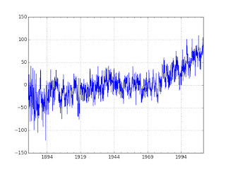
It turns out they are statistical tests for that. We used dataset from GISS, temperature anomalies between 1880-2010 are captured here (anomalies are relative to the 1951-80 base period means). We used ADF test, the implementation we used is able to test for combination of hypothesis’ – pure RW, no pure RW no drift no trend, etc. Well, the test shows GISS data is not pure random walk, it is random walk with a trend (trend stationarity).
At this point deniers can try to shift gears and argue for mean-reversion (opposite of random walk), “what goes up must come down and vice versa” surely there is a certain amount of mean-reversion in this data. Traders love mean-reversion by the way, and if you could trade on temperature data wouldn’t you? Hell yeah! Buy low in the winter, sell high in the summer. But the deniers can never prove full-mean reversion on this data, and since the ADF test blew through all threshold values all indicators are screaming out a trend.
There are other methods as well, such as cointegration, that took care of the attribution part of the equation. That final analysis was the one that truly sealed the deal. It is game-over for the deniers.
Temparature anomaly data from GISS, anomalies are relative to the 1951-80 base period means.
import pandas as pd
dfclim = pd.read_csv('climate-giss.csv',index_col=0,parse_dates=True)
dfclim.Temp.plot()
plt.hold(False)
plt.savefig('climate_01.png')
plt.hold(False)
ACF / PACF
import statsmodels.api as sm
plt.hold(True)
sm.graphics.tsa.plot_acf(dfclim.Temp.values.squeeze(), lags=50)
plt.savefig('climate_02.png')
plt.hold(False)

import statsmodels.api as sm
plt.hold(True)
sm.graphics.tsa.plot_pacf(dfclim.Temp, lags=50)
plt.savefig('climate_03.png')
plt.hold(False)

Dickey Fuller Tests
%load_ext rpy2.ipython
%R library(urca)
series = dfclim.Temp
%R -i series
%R  adf <- ur.df(series, type = 'trend',selectlags="AIC")
%R -o adfout adfout <- summary(adf)
print adfout
###############################################
# Augmented Dickey-Fuller Test Unit Root Test #
###############################################

Test regression trend


Call:
lm(formula = z.diff ~ z.lag.1 + 1 + tt + z.diff.lag)

Residuals:
    Min      1Q  Median      3Q     Max
-80.967  -9.868   0.214  10.370  85.279

Coefficients:
              Estimate Std. Error t value Pr(>|t|)
(Intercept) -10.578706   1.163642  -9.091   <2e-16 ***
z.lag.1      -0.277517   0.020894 -13.282   <2e-16 ***
tt            0.014425   0.001428  10.105   <2e-16 ***
z.diff.lag   -0.224780   0.024657  -9.116   <2e-16 ***
---

Residual standard error: 16.81 on 1562 degrees of freedom
Multiple R-squared:  0.2205,	Adjusted R-squared:  0.219
F-statistic: 147.3 on 3 and 1562 DF,  p-value: < 2.2e-16


Value of test-statistic is: -13.2819 58.8243 88.2169

Critical values for test statistics:
      1pct  5pct 10pct
tau3 -3.96 -3.41 -3.12
phi2  6.09  4.68  4.03
phi3  8.27  6.25  5.34
import statsmodels.api as sm
arima_mod1 = sm.tsa.ARIMA(dfclim.Temp, (1,1,2)).fit()
print arima_mod1.aic
13238.7766703
arima_mod2 = sm.tsa.ARIMA(df.Temp, (2,0,1)).fit()
print arima_mod2.aic
13277.4918251
import statsmodels.api as sm
dfclim = pd.read_csv('climate.csv',sep='\s*',header=None,names=['Temp'])
df = dfclim.copy()
df.index = pd.Index(sm.tsa.datetools.dates_from_range('1880m1', '2010m8'))
df.to_csv('climate2.csv')
print dfclim.head(4)
   Temp
0   -42
1   -17
2   -21
3   -33
from numpy import log, polyfit, sqrt, std, subtract

def hurst(ts):
    lags = range(2, 100)
    tau = [sqrt(std(subtract(ts[lag:], ts[:-lag]))) for lag in lags]
    poly = polyfit(log(lags), log(tau), 1)
    return poly[0]*2.0

print hurst(dfclim.Temp)
0.040611546891
Carbon and Temparature
Plotted carbon levels in the atmosphere and global temparature, trying to gauge a relation between the two. Carbon data comes from here.
import urllib.request as urllib2, io
import pandas as pd

url = "ftp://aftp.cmdl.noaa.gov/products/trends/co2/co2_mm_mlo.txt"
r = urllib2.urlopen(url).read()
file = io.BytesIO(r)
df = pd.read_csv(file,comment='#',header=None,sep='\s*')
g1 = df.groupby(0)[3].mean()
dfc = pd.read_csv('climate-giss.csv',index_col=0,parse_dates=True)
dfc['year'] = dfc.apply(lambda x: x.name.year,axis=1)
dfc['mon'] = dfc.apply(lambda x: x.name.month,axis=1)
dfc['TempC'] = ((dfc.Temp-32)*5.0)/9.0
g2 = dfc.groupby('year')['TempC'].mean()
g = pd.concat([g1, g2], axis=1).dropna()
g.columns = ['Carbon','Temparature']

ax1 = g['Carbon'].plot(color='blue', grid=True, label='Carbon (ppm)')
ax2 = g['Temparature'].plot(color='red', grid=True, label='Temparature (C)',secondary_y=True)
h1, l1 = ax1.get_legend_handles_labels()
h2, l2 = ax2.get_legend_handles_labels()
plt.legend(h1+h2, l1+l2, loc=2)
plt.savefig('carbontemp.png')
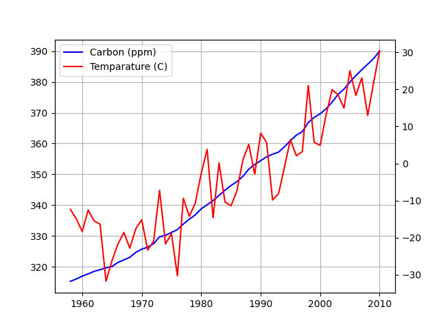
Strong correlation, but does that mean causation?
Running a Granger causality test, which tries to reject the hypothesis that second time series (carbon) does not cause the first series (temparature).
import statsmodels.tsa.stattools as t
res = t.grangercausalitytests(g[['Temparature','Carbon']],maxlag=3)
print (res)
Granger Causality
number of lags (no zero) 1
ssr based F test:         F=34.1256 , p=0.0000  , df_denom=49, df_num=1
ssr based chi2 test:   chi2=36.2149 , p=0.0000  , df=1
likelihood ratio test: chi2=27.4837 , p=0.0000  , df=1
parameter F test:         F=34.1256 , p=0.0000  , df_denom=49, df_num=1

Granger Causality
number of lags (no zero) 2
ssr based F test:         F=11.4685 , p=0.0001  , df_denom=46, df_num=2
ssr based chi2 test:   chi2=25.4301 , p=0.0000  , df=2
likelihood ratio test: chi2=20.6321 , p=0.0000  , df=2
parameter F test:         F=11.4685 , p=0.0001  , df_denom=46, df_num=2

Granger Causality
number of lags (no zero) 3
ssr based F test:         F=5.3519  , p=0.0032  , df_denom=43, df_num=3
ssr based chi2 test:   chi2=18.6695 , p=0.0003  , df=3
likelihood ratio test: chi2=15.8641 , p=0.0012  , df=3
parameter F test:         F=5.3519  , p=0.0032  , df_denom=43, df_num=3
{1: ({'ssr_ftest': (34.12560659900744, 4.0997667759058264e-07, 49.0, 1), 'ssr_chi2test': (36.214929452007894, 1.7671160136200755e-09, 1), 'lrtest': (27.483689910062537, 1.584249217215468e-07, 1), 'params_ftest': (34.12560659900759, 4.099766775905632e-07, 49.0, 1.0)}, [<statsmodels.regression.linear_model.RegressionResultsWrapper object at 0x7f54b4946518>, <statsmodels.regression.linear_model.RegressionResultsWrapper object at 0x7f54b4946630>, array([[0., 1., 0.]])]), 2: ({'ssr_ftest': (11.468479812558117, 9.099787320501968e-05, 46.0, 2), 'ssr_chi2test': (25.43010741045496, 3.005538798970397e-06, 2), 'lrtest': (20.632104155556192, 3.309752413988568e-05, 2), 'params_ftest': (11.468479812556222, 9.099787320513459e-05, 46.0, 2.0)}, [<statsmodels.regression.linear_model.RegressionResultsWrapper object at 0x7f54b4946898>, <statsmodels.regression.linear_model.RegressionResultsWrapper object at 0x7f54b49469b0>, array([[0., 0., 1., 0., 0.],
       [0., 0., 0., 1., 0.]])]), 3: ({'ssr_ftest': (5.351917020399335, 0.003196324450636187, 43.0, 3), 'ssr_chi2test': (18.669477978137216, 0.0003199702464963456, 3), 'lrtest': (15.864090764221487, 0.0012091064117637019, 3), 'params_ftest': (5.351917020398325, 0.0031963244506395256, 43.0, 3.0)}, [<statsmodels.regression.linear_model.RegressionResultsWrapper object at 0x7f54b4946c50>, <statsmodels.regression.linear_model.RegressionResultsWrapper object at 0x7f54b4946d68>, array([[0., 0., 0., 1., 0., 0., 0.],
       [0., 0., 0., 0., 1., 0., 0.],
       [0., 0., 0., 0., 0., 1., 0.]])])}
The hypothesis is rejected at a very strong level. Carbon content in atmo did cause a global increase in temparature.