Coronavirus Data, Analysis
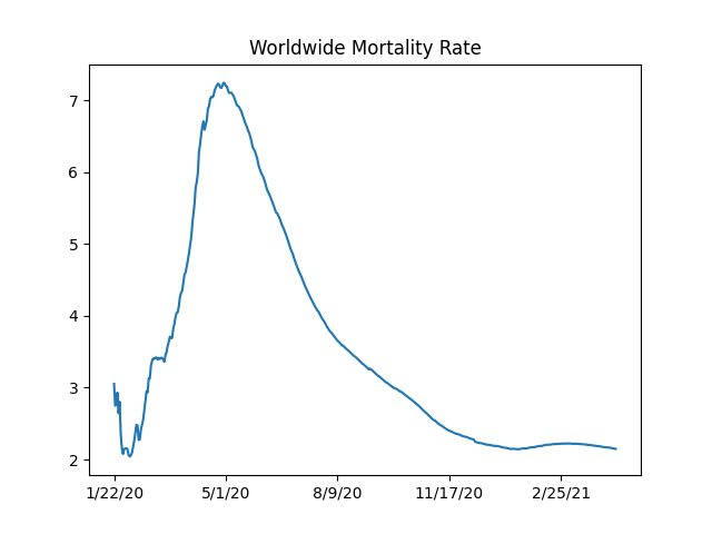
Mortality Rate
Fatality / Cases ratio is around 2.2%, the cases is for people with symptoms. What would be the fatality rate for the broader population? On one of those cruise ships which experienced the epidemic in an isolated environment, they found about 1/3 rd of the people were infected. We can assume the virus reached everyone possible on that ship. 1/3 of mortality rate is nearly 1%. So if given the chance, covid can kill 1% of an entire population. As a reference point, annual growth of world population hovers around the same ratio
Code is from [2]
import util
world_rate_df = util.mortality_rate()
world_rate_df['deaths / 100 confirmed'].plot(title='Worldwide Mortality Rate')
plt.savefig('mort.png')
4/12/21    2.155482
4/13/21    2.152956
4/14/21    2.150022
4/15/21    2.146887
Name: deaths / 100 confirmed, dtype: float64
The SIR Model
\[\frac{ds}{dt} = -\beta s i\] \[\frac{di}{dt} = \beta s i - \gamma i\] \[\frac{dr}{dt} = \gamma i\]Where does $R_0$ come from? Epidemic occurs if # of infected ppl increase, meaning $di / dt > 0$. That means (from 2nd eq above)
\[\beta si - \gamma i > 0 \implies \frac{\beta s i }{\gamma} > i\]Then,
\[\frac{\beta s }{\gamma} > 1\]At the beginning of the epidemic everyone is susceptible, so $s \approx 1$. Substitute $s=1$
\[\frac{\beta}{\gamma} = R_0 > 1\]To find $R_0$ from data, we fit the differential equation system above to data, and using the found $\beta$ and $\gamma$ we calculate $R_0$.
Daily Change
import pandas as pd, util
df = util.get_data()
df['Germany +'] = df['Germany'].diff()
df['UK +'] = df['United Kingdom'].diff()
df['US +'] = df['US'].diff()
pd.set_option('display.width', 2000)
pd.set_option('display.max_columns', None)
print (df[['Germany +','UK +','US +']].tail(10))
Country/Region  Germany +    UK +     US +
4/6/21             7593.0  2404.0  60544.0
4/7/21            30377.0  2797.0  75038.0
4/8/21            26510.0  3124.0  79878.0
4/9/21            23935.0 -4787.0  82698.0
4/10/21           18728.0  2713.0  66535.0
4/11/21            2706.0  1730.0  46380.0
4/12/21           12446.0  3686.0  70230.0
4/13/21           29421.0  2505.0  77878.0
4/14/21           31117.0  2529.0  75375.0
4/15/21           25110.0  2766.0  74289.0
Reproduction Rate $R_t$
This calculation is based on [1]
tau = 7 # length of time window
si_mean = 6.3 # mean of serial interval
si_std = 4.2 # standard deviation of serial interval
conf = 0.95 # confidence level of estimated Reff
c = df['US'].tail(200)
R = util.Reff(c, si_mean, si_std, tau, conf)
df2 = pd.DataFrame(R.T)
print (df2[1].tail(5))
# 0,2 indices 95% conf
df2[1].tail(70).plot()
plt.title('US')
plt.ylim(1.0,1.1)
plt.savefig('Rt-US.png')
195    1.013563
196    1.013634
197    1.013765
198    1.013877
199    1.013940
Name: 1, dtype: float64
Code
References
[1] https://github.com/tt-nakamura/Reff.git
[2] https://notebooks.ai/rmotr-curriculum/analyzing-covid19-outbreak-40c03c06
[4] https://web.stanford.edu/~jhj1/teachingdocs/Jones-on-R0.pdf